Rendering : Making and rendering the origami models

Introduction

Once I had made the stop motion animation, I figured out it would be interesting to make some rendering to achieve the same animation. I had used Blender before but only for its 3D modeling capabilities and I always wanted to learn to use it for proper rendering too. In my head, the project seemed simple, I needed the 3D model, to make a scene for it with lights, cool materials and stuff and to render it. As a beginner I faced many challenges but it was worth it.

3D Models

The first thing on my todo list was to get the 3D models for the base polyhedra, make their augmented version and color their faces.

Getting the base models What I needed were the coordinates of the vertices in a table as well as the faces as a list of the vertices indices, preferably in a proper format for 3D objects like OBJ or OFF. Unfortunately, the "Visual Polyhedra" website [5] did not have the data for any of the Johnson solids mainly because they are less symmetric than the one that are there. Since I knew they were described on the MathWorld web page [7] that is part of the Wolfram environment, I tried to dig into the Wolfram notebooks and that finally led me to this web page of the documentation: [6]. With this piece of information I made a script on the Wolfram Development Platform to retrieve the data I needed.

Then, I wrote a piece of Python code to make obj files out of the output of the Wolfram script and it was done.

Edit: the "Visual Polyhedra" website [5] will soon provide visualizations for the Johnson solids.

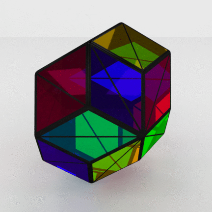
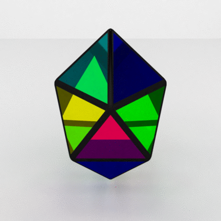
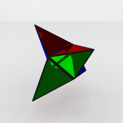
Augmentation The next step was to get the augmented models. Again, I wrote a piece of Python code for this purpose where I could control the side-to-edge ratio I desired for the pyramid isosceles triangles. For the rhombic polyhedra, I made something simple. The base faces are kept flat and the triangular faces of the pyramid are not isosceles triangles anymore. I am still in the process of figuring out the maths to get an augmented 3D model similar to the origami model. A zip archive is available here with the base and augmented models as well as the color textures for blender.

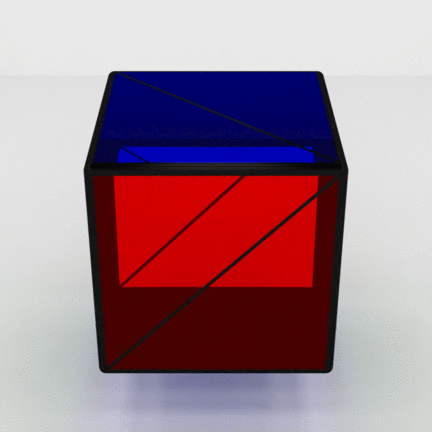
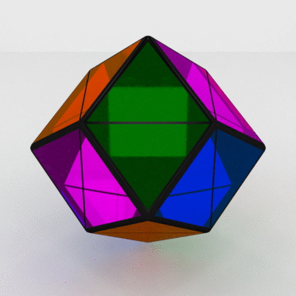
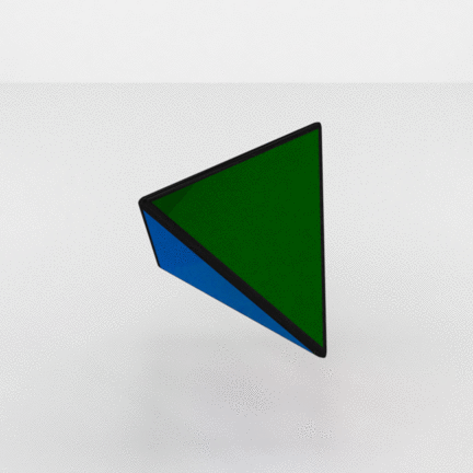
Color attribution Then, the issue was to give each face its proper color by respecting the rules I had set when working on the origami models. To sum up, I wanted the minimal edge coloring of the base model so that no two edges belonging to the same face have the same color. Minimal meaning with the least number of colors. I already had the manual solutions I had used for the origami models but I wanted to do the things automatically this time. I looked up for a Python graph library that would be able to colorize graphs and found NetworkX [4].

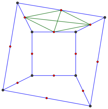
Any colorization problem in graph theory works on the vertices, so I had to work out the proper graph that would express my specific constraints and feed it to the colorization algorithm. In this graph, the nodes are the edges of the base polyhedra mesh. Let’s call this graph the edge graph. To connect the nodes, consider the subset of nodes that belongs to a face. Since all the corresponding edges have to be of a different color, it means that their nodes are all linked together in the edge graph. This subset of nodes forms a complete graph. Repeat the process for each face and the edge graph is done, see Figure 1.

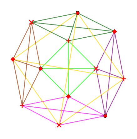
I also ended up coloring the base models but this time such that each of the face around a vertex is of a different color. In this case, each node in the graph represents a face and the nodes corresponding to the faces around a common vertex forms a complete graph. Looping over the vertices gets the things right, see Figure 2.

Finding the minimal coloring of a graph is a NP problem. The function greedy_color of the NetworkX library offers several algorithms to color a graph but do not guarantee that a minimal number of color is used. So, I tested every algorithm and kept the solution giving out the minimal number of color. It worked for all the polyhedra I wanted. TODO: code ?

Face coloring with Blender Usual file formats for 3D objects, like OBJ, OFF stores the properties of the models (color, texture coordinates, normals, ...) at the vertex level and not at the face level. The main hack to get per-face color is to duplicate each vertex for each of the face it belongs too and to set the properties of the vertices of the same face to be equal. This way, colors are interpolated correctly on the face when viewing with MeshLab for instance. The main issue with this hack, apart form the unnecessary replicating, is that all the faces in the model are independent from each other which, for instance, breaks some of the Blender modifier tools.

After looking up for some solution for a while, I tested the PLY format which does accept color attribution per face and is generally more flexible than OBJ and OFF formats. However, Blender would not read the additional data correctly. Finally, I found a great answer in a closely related Blender question about per face vertex coloring [3]. It required a bit of scripting (which I did not know about at all) but I managed to adapt the idea to my need. I am really grateful to the writer of this solution. By the way, it necessitates to use Cycles as the renderer.

Edit: Later, I found an alternative way without using Cycles but that’s for another post.

Single Model Scene

With the model and the coloring ready, what was left was to make the actual scene. Roughly, the scene is made of a room with white walls, a white ground and a black ceiling. In the center stands the model. The camera view is centered on the model and rotates around it with a linear angular increment depending on the number of frames (72 or 360) [1]. The lights are actually a 5x5 array of squares near the ceiling. I used ambient occlusion.

Materials The material of the walls, ground and ceiling uses the diffuse BSDF node. The lights are a single object with an emission shader.

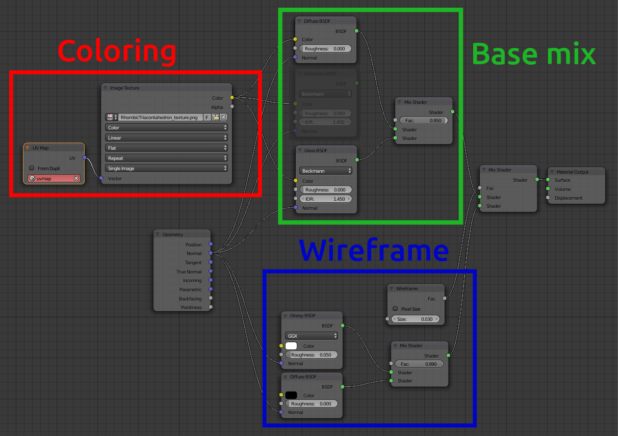
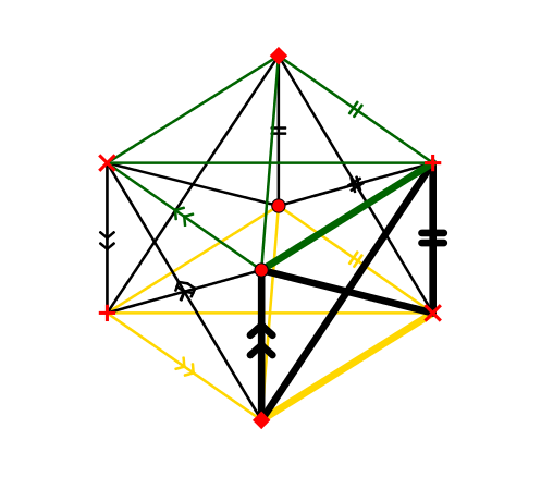
The material for the model is more complex. After testing different kinds of material, I found that having a glass material would be kind of cool and visually interesting. The material is actually a mix of the Glass BSDF node and the Diffuse BSDF node (95-5), see Figure 3. I also wanted to show the edges distinctively, so i used the Wireframe node and applied a modifier to the object to have large edges and smooth transitions between faces. The modifier is set apart in the script. The material for the wire frame is a mix of a white glossy BSDF and black diffuse BSDF (1-99).

Scripting I wanted to have the same scene for all the models and a way to run the rendering automatically so that there is only one model in the room at a time so I had to make some script. I made it so that it can be run either directly from the command line or from the Blender text editor with a boolean flag.

In the script, the models to be rendered have to be indicated. This could go in a separate config file. Then, each model is rendered in a loop where its position, coloring, material and modifier are defined. The choice between rendering a single image or the full animation is decided with some flags.

Other details The parameters for the render such as the image resolution, number of samples and bounces have to be modified in the blender scene directly.
I also chose to use some denoising in order to reduce the number of samples and consequently the rendering time. It works well on the diffuse walls but creates some small artifacts on the light reflections by the model.
I later found about the Fresnel node to get a more realistic material for the model as well as a technique to simulate chromatic aberrations [2] but I did not use them.

The blender files are available here. I made a git for it already but its private.

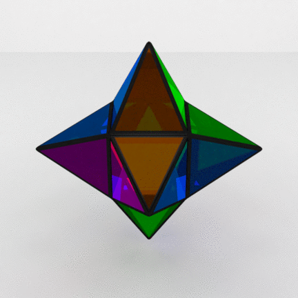
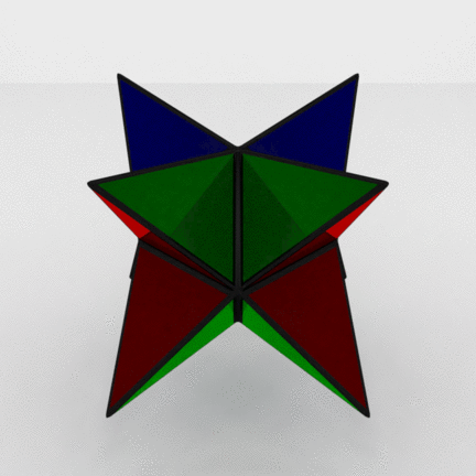
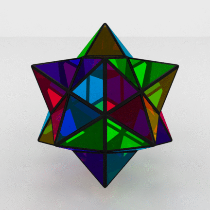
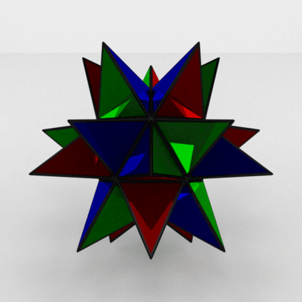
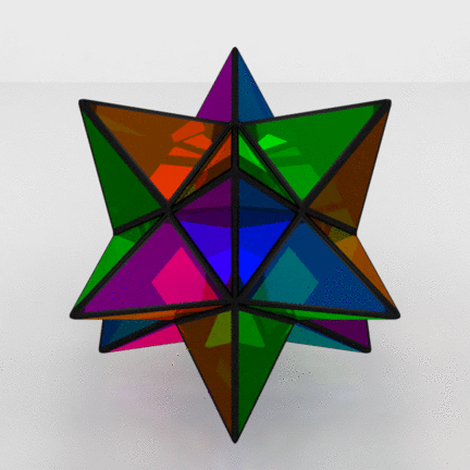
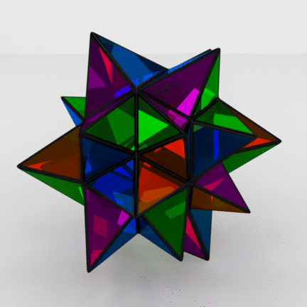
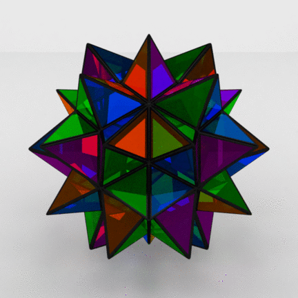
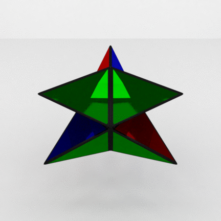
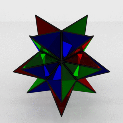
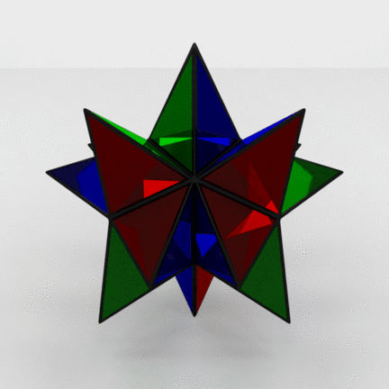
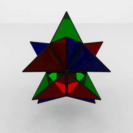
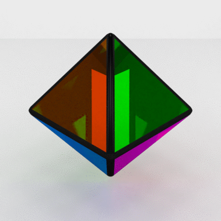
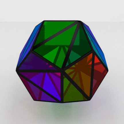
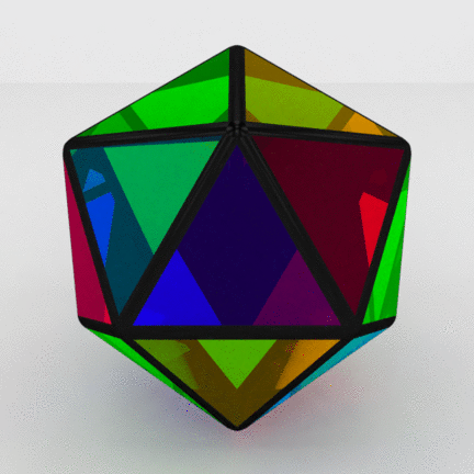
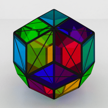
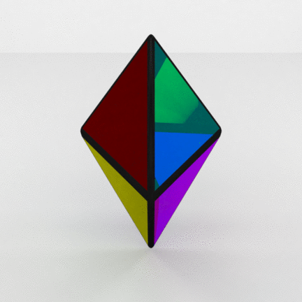
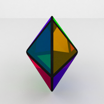
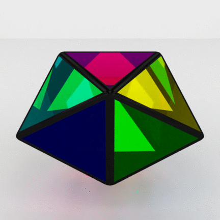
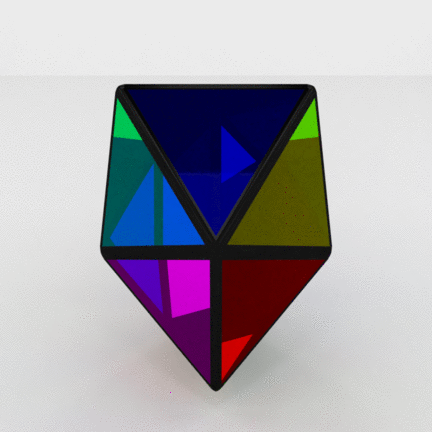
Gallery

The final high quality rendering of these animations was realized by a friend of mine. Kudos to him. As for the stop motion animation, I used ImageMagick and Kdenlive to make the animated pictures and videos. Clicking on a picture will open its HD animated version.

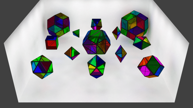
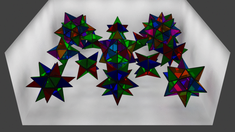
Many models scenes Moreover, I made two other scenes. The environment for both is the same room but I had to adjust the camera position. In the first, I have grouped all the augmented models and, in the second, all the base models. These two scenes do not need the script to be rendered. Here are the animated renders.

Stand alone models

Ping pong animation This has nothing to do with table tennis. I just thought that having additional animation alternating between the base and the augmented model would be cool.

References

[1] How can i animate the camera in a perfect circular rotation around a fixed position? https://blender.stackexchange.com/questions/3476/how-_can-_i-_animate-_the-_camera-_in-_a-_perfect-_circular-_rotation-_around-_a-_fixed-_posit. Accessed on 08-15-2018.
[2] Light spectrum dispersion effect in blender? https://blender.stackexchange.com/questions/1602/light-_spectrum-_dispersion-_effect-_in-_blender. Accessed on 08-16-2018.
[3] Per face vertex coloring. https://blender.stackexchange.com/questions/80205/per-_face-_vertex-_coloring. Accessed on 08-14-2018.
[4] NetworkX Developers. Networkx docs. https://networkx.github.io/documentation/stable/index.html. Accessed on 08-15-2018.
[5] David I. McCooey. Visual polyhedra. http://dmccooey.com/polyhedra/. Accessed on 08-11-2018.
[6] Wolfram Development Team. Wolfram language documentation center - polyhedrondata. https://reference.wolframcloud.com/cloudplatform/ref/PolyhedronData.html. Accessed on 08-13-2018.
[7] Eric W. Weisstein. Johnson solid. http://mathworld.wolfram.com/JohnsonSolid.html. Accessed on 08-13-2018.